Home •
People •
Courses •
Program •
Research •
Clinic •
Goals •
Kiosk •
News
Understanding Basic Statistics •
Fitting •
Exercise •
Excel •
Igor •
Kaleidagraph •
Origin •
Power Laws •
Dimensional Analysis
Fitting Exercise
This exercise will help you learn how to use
Kaleidagraph or Origin to plot and analyze data.
Introduction
 In 1798 Henry
Cavendish conducted an experiment to “weigh the earth.” (Actually, he was interested
in the Earth's density, from which he hoped to estimate the time Earth took
to cool from a fiery beginning.) He did this by measuring the shift in the
equilibrium position of a small dumbbell suspended
from a
torsion fiber caused by two cannonballs. The balls were placed near the dumbbell
so as to make it twist. From the spring constant of the fiber, the geometry
and masses of the dumbbell and cannonballs, and the magnitude of the angular
shift the cannonballs cause, it is
possible to measure the value of G, the universal constant of gravitation.
Combined with knowledge of the radius of the earth and the
local value of (little) g, the local acceleration due to gravity,
one can deduce the mass of the earth.
In 1798 Henry
Cavendish conducted an experiment to “weigh the earth.” (Actually, he was interested
in the Earth's density, from which he hoped to estimate the time Earth took
to cool from a fiery beginning.) He did this by measuring the shift in the
equilibrium position of a small dumbbell suspended
from a
torsion fiber caused by two cannonballs. The balls were placed near the dumbbell
so as to make it twist. From the spring constant of the fiber, the geometry
and masses of the dumbbell and cannonballs, and the magnitude of the angular
shift the cannonballs cause, it is
possible to measure the value of G, the universal constant of gravitation.
Combined with knowledge of the radius of the earth and the
local value of (little) g, the local acceleration due to gravity,
one can deduce the mass of the earth.
Data have been collected for the angular position of the dumbbell as a function
of time, and are available by (right) clicking
here. Right-click (or control-click) and save the data to a file, for opening
in your data analysis program of choice (this preserves the
tabs which delimit columns in the file). Alternatively, you
may retype them or select them in your browser for pasting into the data analysis
program. However, in the latter case be careful that the data
show up as numbers in the analysis program, not as text.
The motion is described by a damped sinusoid. Its functional form is
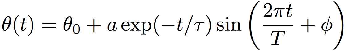
where the quantities in the equation are defined by
| a |
(angular) amplitude of oscillation |
| T |
period of oscillation |
| φ |
initial phase of the motion |
| τ |
exponential decay time of the motion |
| θo |
shift in the equilibrium position of the dumbbell |
There are six steps to this exercise. Each task has a help link for Kaleidagraph
and Origin, which you may obtain by clicking the link.
- Load the data ( KG Help, Origin
Help ).
- Plot the data ( KG Help, Origin
Help ).
- Add error bars ( KG Help, Origin
Help )
to the plot.
Do the data look like they could represent the motion of a twisting
pendulum slowed down by air resistance? Save the plot.
- Define a fitting function. ( KG
Help, Origin Help) that calculates a damped sinusoid.
In Kaleidagraph, be careful to check whether you wish the
trigonmetric function
to be evaluted in radians or degrees. Also be sure to check
the Weight Data box in the fit function dialog box.
Fit your data. Be very careful to choose good guesses for your parameters. If
you don't, you will very likely get an error like Singular Matrix Error or
some such "useful" diagnostic information. In Origin, you can press
the Update Plot button to see how you are doing. In Kaleidagraph, there
is no such facility.
- When you have finished the fitting procedure, you should
have a graph showing the data with error bars, the fitted curve,
and some fit information ( KG
Help, Origin Help ).
When you perform a proper χ2 fit,
the error associated with each fit parameter gives you a sensible
estimate of the accuracy of the parameter, as determined by
the fitting operation. That's pretty nice. Have a look at your
graph and see how well you could eyeball the angular offset.
It's tough!
If you're curious for more details about the fitting operation, click here.
- Lastly, print out a copy of the graph ( KG
Help, Origin Help
). Make the plot area about 4 inches wide by 3 inches high.
This is a nice size for taping into a lab
notebook.
The function χ2 is defined by
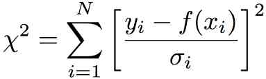
which looks more frightening than it is. This function adds up the differences
between each data point and the fitted curve, symbolized here by f.
In this equation, the xi are the values of the independent
variable. In this example, the independent variable is time. The yi are
the values of the dependent variable, which is θ in this problem.
The sum is over the N data points.
There are two subtleties. First, the differences are squared, to make them
all add up positively. If they weren't, the average would be zero! Second,
each difference is divided by the uncertainty of the data point. This means
that you get penalized a lot when the curve is far from a "good" data point
(that has small uncertainty), and not much at all when the curve is far from
a "lousy" data point (that has a large uncertainty).
Since χ2 is the sum of nonnegative quantities, the smallest
value it can have is zero. This happens when the curve goes through each and
every data point. You might think that this is the best you can do, but you'd
be wrong. It means either that you cheat or that you're really sloppy! (Newton
cheated with his data and got away with it, because nobody was very sophisticated
about this sort of thing when Newton was working out the foundations of mechanics.)
Real data have random noise at some level, and this means that they will virtually
never lie right on the curve. The uncertainty of a data point is an estimate
of the likely discrepancy between the point and its true value. Roughly speaking,
a typical data point should be within about one uncertainty ("one error bar")
from its true value. This means that each data point should contribute a value
of about one to the sum. So the sum should be about N.
It is often more convenient to compute the "per point" value of χ2.
This is called the reduced χ2 or χ2 per degree
of freedom. It turns out that the best procedure is to divide χ2 not
by the number of data points, N, but by N - m, where m is
the number of fitting parameters. The number you get should be in the ballpark
of unity for a good fit. If it's much smaller than you probably overestimated
your errors. If it's much bigger, you may have underestimated your errors or
your model may not describe the data very well.
Origin reports a value of chisq. Don't be fooled. It is the reduced χ2.
Kaleidagraph reports a value of chi^2. It is χ2.
To get the reduced χ2, divide by the number of degrees of freedom
(N - m).
Understanding Basic Statistics •
Fitting •
Exercise •
Excel •
Igor •
Kaleidagraph •
Origin •
Power Laws •
Dimensional Analysis
 |
Copyright ©
Harvey Mudd College Physics Department
241 Platt Blvd., Claremont, CA 91711
909-621-8024
http://www.physics.hmc.edu/
WebMaster (at) physics.hmc.edu
Last modified: 26 August 2012
|