Jet Propulsion Laboratory, California Institute of Technology
Pasadena, CA 91109
Bahram Nour-Omid
Lockheed Palo Alto Research Laboratory
Palo Alto, CA 94304
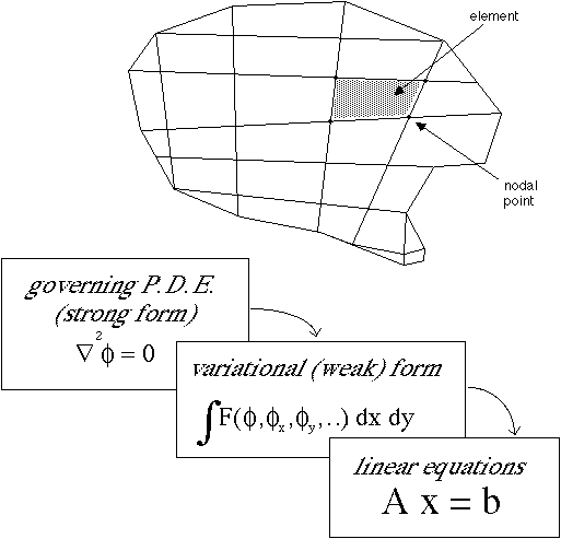
Figure 1 - Finite Element Discretization
The finite element method is used for the approximate solution of partial differential equations that arise in engineering and scientific contexts[1]. As shown schematically in Fig. 1, the method employs a spatial discretization of a continuous domain. In general, the domain is represented by a mesh of nodal points, and the polygonal (or polyhedral) regions delimited by this gridding are the elements, from which the finite element method derives its name.
The original governing differential equation or so-called strong form can be shown to be equivalent to an integral variational weak form statement of the problem. This weak form in turn is applied to the discretized domain through the introduction of a set of approximate nodal basis functions. This discretization of the weak form results in a discrete set of unknown coefficients which are related by a system of linear algebraic equations. Thus, the finite element method involves the construction and solution of a matrix system whose rank is equal to the total number of unknown nodal degrees of freedom.
The matrix which results from this finite element approximation is in general sparse, with an irregular clustering of non-zero elements near the diagonal. The particular structure and non-zero column profile of the stiffness matrix is dictated by the spatial connectivity of the problem domain. The matrix contains non-zero entries connecting only those degrees of freedom which share a common finite element in the domain discretization. This spatial locality results from the element-wise assembly of the stiffness matrix. Element-level matrix contributions are obtained by integration of basis functions over the volume of individual elements, which are in turn additively assembled into the global matrix. It is just this element-wise separability of the stiffness matrix which lends itself naturally to a domain decomposition approach to parallelizing finite element calculations.
Interprocessor communication is invoked in order to exchange this "boundary" information and obtain a global solution. While this model of domain decomposition is particularly suited to the distributed memory machine model, it should be noted that it is equally useful for large-node multiprocessors in a shared or common memory environment. In such cases, it is
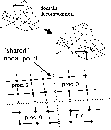
Figure 2 - Domain Decomposition
Examining the finite element decomposition in more detail, we see that elements become the exclusive responsibility of exactly one processor. While nodal point information is also distributed among processors, it is seen that some nodal points fall on boundaries and are in some sense shared by two or more processors. In such cases, it is necessary to devise a bookkeeping scheme to ensure consistent treatment of these degrees of freedom. In particular, one and only one processor must be identified as "responsible" for accumulating contributions to a given shared degree of freedom. Conversely, the "subordinate" processors sharing a given nodal point must supply the missing information needed to complete a given operation. This bookkeeping however, will turn out to fit quite naturally within the context of conventional (sequential) finite element programming methods. Before examining this "management" task in detail though, it will be helpful to look at the kinds of linear algebraic methods it will be necessary to implement.
One common and well-understood approach to the solution of large linear systems is direct elimination. Variants of Gaussian elimination which exploit the limited non-zero column height of the sparse finite element matrix are widely used. Useful because of their comparative robustness and cost-predictability, direct elimination methods can be prohibitively expensive for systems of large rank and bandwidth, such as arise from large three-dimensional domains.
We can make use of an adaptation of direct methods to the domain-decomposed parallel problem. In this approach, each processor eliminates the "interior" degrees of freedom of its subdomain in terms of the shared nodal values. This "substructure elimination" step proceeds independently in each processor without communication. At its conclusion each processor is left with a partial matrix describing the mutual interactions of the reduced system of equations. These partial matrices can be thought of as "superelement" matrices by analogy with the element matrices which made up the original unreduced stiffness matrix.
At this point, it is necessary for the processors to communicate their matrix elements in order to further reduce the system and ultimately recover the solution. One possible way to accomplish this (which is natural for a hypercube comprised of 2**N processors) is to have half of the processors turn over their subdomains to a neighbor for further reduction, and proceed recursively until the entire domain resides in a single processor. While this has the unattractive property of rendering processors idle, the vast majority of the computational work is generally performed in the first parallel stage, so that the overall concurrent efficiency is minimally impacted.
We may note in passing that alternate methods for concurrent direct elimination exist which do not use such a domain decomposition, but rather break the problem up by matrix rows and columns. While such methods have proven practical for various kinds of general matrices, they do not exploit the particular sparse local structure imparted by the underlying finite element domain. We believe that practical finite element applications for concurrent processing will center on methods based upon domain decomposition rather than general "matrix library" methods which recognize no underlying locality in the matrix structure.
An alternative approach to linear equation solving which also employs domain decomposition is the use of iterative methods. Solvers like the preconditioned conjugate gradient (PCG) method proceed by iterative improvement toward an approximate solution[2]. A good deal of previous work has gone into consideration of such methods for parallel implementation because of two considerations. Firstly, the computational cost (per iteration) of such methods increases much less rapidly with increasing domain size than is the case for direct methods. Secondly, the iterative methods are most amenable to domain decomposition, requiring only minimal communication of boundary information between processors.
Unfortunately, iterative methods are not particularly robust, in the sense that their convergence properties are highly problem-dependent and difficult to guarantee with any single preconditioner. In the work discussed below, we have taken a hybrid approach which seeks to combine many of the advantages inherent in both direct and iterative methods. By employing direct elimination methods on the subdomain interiors, and PCG iteration on the remaining boundary system, a comparatively efficient and robust solver is obtained. In the iterative component of the method, the system rank is a small fraction of that of the full unreduced system. This has been shown[3] to reduce the matrix condition number, and therefore enhance the convergence of PCG. In the direct component of the method, the costs are limited to those associated with reduction of a small subdomain. Therefore, if the number of processors is increased in direct proportion to the problem size, the cost associated with elimination remains constant, in contrast with the cost of an elimination-only scheme which would increase faster that in simple proportion to problem size.
Since the number of steps required for convergence of the iterative component is difficult to predict, we cannot state unequivocally that the hybrid method will be optimal under all circumstances. Experience with the method however, has shown that for a given problem there exists an optimal number of processors to minimize the total cost of the hybrid method, and that this number increases with increasing problem size. Thus we may surmise that as problem size and number of processors increase together (over some range) the hybrid method will at least remain competitive with pure iterative and direct methods and perhaps surpass them.
All of the parallel solution algorithms discussed above require some interprocessor communication activity. It is possible to generally characterize the kinds of communication tasks called for and to devise generic procedures for performing them. In broadest outline, the communication tasks called for in a static decomposition with no adaptive regridding are a priori predictable, so that the individual processes can execute in parallel, scheduling communication with other processors and maintaining "loose synchronization" by following a predetermined "script". (The more general case of dynamic decomposition can be thought of as an extension of this case, with the dominant periods of loosely synchronous message passing interspersed with infrequent episodes of "unstructured" communication during which regridding and/or decomposition adjustment occur.)
Looking more specifically at the problems considered here, two generic linear algebraic operations dominate the tasks which require communication. These tasks are scalar products and matrix-vector products (Fig. 3). In the former case,
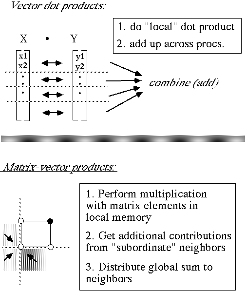
Figure 3 - Operations requiring communication
Only a slight generalization of this concept of mapping arrays is required to manage communicated nodal values. We introduce two new mapping arrays to which we refer as the send index and the accumulate index (Figs. 4a, 4b). These indices consist of lists, maintained separately in each processor, which contain the mapping of each shared degree of freedom into destination processor and equation number. The send index in each processor contains, for each shared nodal point for which responsibility is elsewhere, the unique remote "address" to which its contribution should be sent. The accumulate index on the other hand, contains (for each degree of freedom of local responsibility) all the addresses of incoming contributions, which are needed for final redistribution of the result.
The simple case illustrated schematically in Fig. 4 is that of a corner nodal point shared by four processors. It should be noted however, that just as the finite element formalism is sufficiently general to handle irregularly shaped and even multiply connected domains, our mapping index constructs allow the transparent treatment of arbitrary configurations of shared corners and edges. All that is assumed in this approach is availability of unrestricted processor-to-processor message passing. We examine next the significance of this and other assumptions regarding the interprocessor communication facilities.
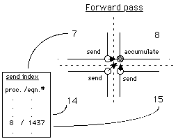
Figure 4(a) - "Send" index for interprocessor communication
(1) Global data broadcast/combine
(2) Processor-to-processor message posting
(3) Intermittent process synchronization
These three requirements turn out not to be particularly restrictive, and can be realized not only in the distributed memory machine environments to which this work has been primarily directed, but in shared memory machines as well.
In the hypercube environment, routing and branching algorithms which use the connections of the Boolean N-cube can be used to implement efficient and elegant communications. Fox et al.[4] have described the combine and crystal router algorithms which satisfy requirements (1) and (2) above, and have been employed in the current work on the Mark III hypercube. The third requirement of coarse process synchronization is satisfied automatically in a polled communication environment (as with the Mark III Crystalline OS) and is easily implemented in an interrupt-driven communication system (e.g. Mark III Mercury OS).
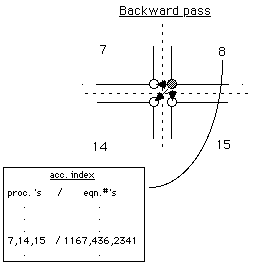
Figure 4(b) - "Accumulate" index for interprocessor communication
While we have gone to some length to demonstrate the generality of the parallel FEM approach, perhaps of greater significance is the ease with which these ideas are incorporated into conventional sequential finite element work. As already discussed, the equation bookkeeping associated with the "accumulate" and "send" indices amounts to a natural extension of the usual finite element domain-to-matrix mapping structures. On the algorithmic level as well, the changes in going to the parallel FEM are largely incremental and localized, rather than radical and comprehensive. For example, Fig. 5 outlines the concurrent preconditioned conjugate gradient algorithm in the present context. The few steps in which this differs from the sequential version are shown shaded. These communication tasks (which contain all of the machine-specific interprocessor activity) are isolated from the familiar calculation tasks. Thus the equivalent sequential procedure is recovered by simply deleting the shaded steps.
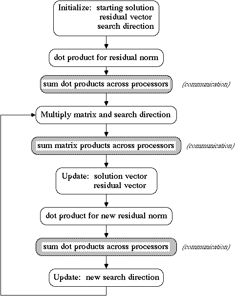
Figure 5 Conjugate Gradient Algorithm in Concurrent FEM
The earliest and most straightforward applications of these ideas have involved static linear finite element analysis. Two-dimensional elastostatics problems in continuum and structural mechanics have been effectively and efficiently treated by these methods on the JPL/Caltech Mark III hypercube computer.
A typical problem solved in this work is shown in Fig. 6. The illustrated grid represents a cross section through an axisymmetric rocket nozzle component. The example is useful in illustrating some of the issues involved in the practical implementation and use of parallel FEM techniques.
The grid consists of 6216 plane strain elements, which together include 13,238 displacement degrees of freedom. Using a 32-processor Mark III hypercube and the hybrid direct/PCG method, this static problem was solved in 141 seconds. This represents an approximately 95% efficient utilization of the ideal 32-fold speedup (over one processor) possible on this machine.
Original figure unavailable at this time
Figure 6 Example 2-D Finite Element Grid Solved on Mark III Hypercube
While the robustness of the interprocessor communication method guarantees that even a rather crude domain partition will be correctly solved, efficiency considerations dictate that the partition should be chosen judiciously. The most important consideration in this regard is interior work load balance. This means assigning equal numbers of degrees of freedom to each processor. Of less, but still significant importance are the numbers of interprocessor boundary points. It is clearly desirable from a computational efficiency standpoint to minimize the number of communicated degrees of freedom. In the hybrid method, it is also desirable to balance the distribution of shared points, since certain steps of the procedure have costs that depend upon the size of the the reduced system of boundaries, rather than upon the full interior-dominated system. Thus a domain partition that looks quite well-balanced from an element tally standpoint may be severely imbalanced during some phases of the hybrid solution procedure.
The approach to the problem taken here involves passing the problem input data through a preprocessing software stage, which allows for the specification and adjustment of the domain partition. The results described here were obtained with a combination of geometric domain bisection methods and statistical optimization using the method of simulated annealing[7]. These preprocessing steps require a certain amount of human intervention to give satisfactory results, however work is under way to explore means of automating this decomposition/optimization step. It is noteworthy however, that even using the present input preprocessing methods, only a few additional minutes of user manipulation are added to the end-to-end analysis time.
Because of the generality of the methods described here, it has been possible to apply them immediately to a number of problems in nonlinear and time-dependent finite element analysis. Gurnis et al.[8] describe the use of these methods for the simulation of thermally driven convection in geophysical systems. The results obtained are significant, particularly in light of the ill-conditioning problems posed by this class of simulations. Algorithms for the solution of transient viscoplasticity and incompressible Navier-Stokes flow have also been implemented using unchanged the described concurrent FEM software "core". Time-dependent dynamic structural analysis has also been shown to fit well within this parallel FEM environment[9,10]. The range and complexity of problems demonstrated up to this point suggest that the approach can be of considerable practical utility.
This programming approach builds upon (and even exploits) existing FEM paradigms, and may be regarded as a model for the construction of the next generation of finite element analysis packages capable of exploiting computers of parallel architecture. This model generalizes to both distributed and shared memory multicomputers, thus eliminating a degree of machine specificity that might otherwise restrict its general usefulness.
2. Jennings,A., Matrix Computation for Engineers and Scientists, John Wiley and Sons, Chichester, 1977.
3. Li, M. R., B. Nour-Omid, and B. N. Parlett, "A Fast Solver Free of Fill-In for Finite Element Problems", SIAM J. Numer. Anal., Vol. 19, No. 6, Dec. 1982, pp. 1233-1242.
4. Fox, G. C., M. A. Johnson, G. A. Lyzenga, S. W. Otto, J. K. Salmon, and D. W. Walker, Solving Problems on Concurrent Processors, Volume I: General Techniques and Regular Problems, Prentice-Hall, Englewood Cliffs, NJ, 1988.
5. Nour-Omid, B., A. Raefsky, and G. Lyzenga, "Solving Finite Element Equations on Concurrent Computers", in Proceedings of the Symposium on Parallel Computations and their Impact on Mechanics, Boston, December 13-18, 1987, ASME, 1988.
6. Lyzenga, G. A., A. Raefsky, and B. H. Hager, "Finite Elements and the Method of Conjugate Gradients on a Concurrent Processor", in Computers in Engineering 1985, vol. 3, Proceedings of the 1985 ASME International Computers in Engineering Conference and Exhibition, Boston, MA, August 4-8, 1985.
7. Flower, J. S. Otto, and M. Salama, "A Preprocessor for Irregular Finite Element Problems", C3P Report No. 292, California Institute of Technology, June 1986.
8. Gurnis, M., A. Raefsky, G. A. Lyzenga, and B. H. Hager, "Finite Element Solution of Thermal Convection on a Hypercube Concurrent Computer", this volume, 1988.
9. Ortiz, M. R. and B. Nour-Omid, "Unconditionally Stable Procedures for Transient Finite Element Analysis", Computer Methods in Applied Mechanics and Engineering, Vol. 58, 1986, pp. 151-174.
10. Ortiz, M. R., B. Nour-Omid, and E. D. Sotelino, "Accuracy of a New Class of Concurrent Algorithms for Transient Finite Element Analysis", to be published in Intl. J. Numer. Meth. Engineering.